# import models
from astroquery.vizier import Vizier
from astropy.table import join, Table, Column
import matplotlib.pyplot as plt
import numpy as np
import plotly.express as px
from plotly.subplots import make_subplots
from mpl_toolkits.axes_grid1.inset_locator import mark_inset
import plotly.graph_objects as go
from astropy.io import asciiHonors: EDA
# query vizier for the catalog
vizier = Vizier()
vizier.ROW_LIMIT = 40000 # max length of catalog is ~30,000
alf_sdss_cat = vizier.get_catalogs("J/AJ/160/271")
data = join(alf_sdss_cat[0], alf_sdss_cat[1], keys="AGC")
data.info()<Table length=31501>
name dtype unit format description n_bad
---------- ------- ------------------- -------- -------------------------------------------------------------------------- -----
AGC int32 [1/749512] AGC catalog identifier 0
Flag uint8 [0/3] Photometry flag (1) 0
ObjID int64 Optical counterpart SDSS DR15 object identifier 1863
RAJ2000 float64 deg {:10.6f} [0.003/360] Right Ascension (J2000) (2) 0
DEJ2000 float64 deg {:9.5f} [-0.21/36.4] Declination (J2000) (2) 0
RVel int16 km / s [-430/17823] HI profile midpoint heliocentric radial velocity 0
Dist float32 Mpc {:5.1f} [0.3/260] Distance from Haynes+, 2018, J/ApJ/861/49 0
e_Dist float32 Mpc {:4.1f} [0/30.9] Uncertainty in Dist 0
gext float32 mag {:5.2f} [0.02/4.44]? Foreground Galactic extinction in SDSS g band (3) 1863
iext float32 mag {:5.2f} [0.01/2.28]? Foreground Galactic extinction in SDSS i band (3) 1863
b/a float32 {:5.2f} [0.05/1]? Axial ratio b/a from SDSS r band 1863
e_b/a float32 {:6.2f} [0.01/865]? Uncertainty in b/a (4) 1863
imag float32 mag {:5.2f} [9.58/30.89]? SDSS i band cmodel magnitude 1863
e_imag float64 mag {:8.2f} [0.01/42134.68]? Uncertainty in imag (4) 1863
Dprop str5 Derived properties (table 2) 0
Sloan str5 Display the online SDSS DR16 for the nearest object 0
Ag float32 mag {:5.2f} [0/1.91]? g band internal extinction factor (1) 3234
Ai float32 mag {:5.2f} [0/0.99]? i band internal extinction factor (1) 3234
iMAG float32 mag {:6.2f} [-24/-10]? Corrected absolute i band magnitude (2) 3234
e_iMAG float32 mag {:5.2f} [0.02/86]? Uncertainty in iMAG 3234
g-i float32 mag {:5.2f} [-1.97/3.8]? Corrected (g-i) color (2) 3234
e_g-i float32 mag {:6.2f} [0.03/220.3]? Uncertainty in g-i 3234
logMsT float32 log(solMass) {:5.2f} [4.49/12.45]? log Taylor method stellar mass (3) 3234
e_logMsT float32 log(solMass) {:6.2f} [0.02/158]? Uncertainty in logMsT 3234
logMsM float32 log(solMass) {:5.2f} [4.4/11.94]? log McGaugh method stellar mass (3) 2203
e_logMsM float32 log(solMass) {:5.2f} [0.01/1.66]? Uncertainty in logMsM 2203
logMsG float32 log(solMass) {:5.2f} [7.37/11.69]? log GSWLC-2 derived stellar mass 16776
e_logMsG float32 log(solMass) {:5.2f} [0/0.25]? Uncertainty in logMsG 16776
logSFR22 float32 log(solMass.yr**-1) {:5.2f} [-5.57/2.17]? log Star Formatation Rate from 22{mu}m unWISE photometry (4) 7606
e_logSFR22 float32 log(solMass.yr**-1) {:5.2f} [0.01/3.6]? Uncertainty in logSFR22 7606
logSFRN float32 log(solMass.yr**-1) {:5.2f} [-3.53/7.88]? log Star Formatation Rate from GALEX NUV photometry (4) 15387
e_logSFRN float32 log(solMass.yr**-1) {:5.2f} [0.02/28.03]? Uncertainty in logSFRN 15388
logSFRG float32 log(solMass.yr**-1) {:5.2f} [-2.94/1.47]? log Star Formatation Rate from GSWLC-2 16776
e_logSFRG float32 log(solMass.yr**-1) {:5.2f} [0.0/1.08]? Uncertainty in logSFRG 16776
logMHI float32 log(solMass) {:5.2f} [3.76/10.94] Haynes+, 2018, J/ApJ/861/49 log HI mass 0
e_logMHI float32 log(solMass) {:5.2f} [0.0/1.12] Uncertainty in logMHI 0WARNING: MergeConflictWarning: Cannot merge meta key 'ID' types <class 'str'> and <class 'str'>, choosing ID='J_AJ_160_271_table2' [astropy.utils.metadata.merge]
WARNING: MergeConflictWarning: Cannot merge meta key 'name' types <class 'str'> and <class 'str'>, choosing name='J/AJ/160/271/table2' [astropy.utils.metadata.merge]
WARNING: MergeConflictWarning: Cannot merge meta key 'description' types <class 'str'> and <class 'str'>, choosing description='Derived properties of cross-listed objects in the ALFALFA-SDSS catalog' [astropy.utils.metadata.merge]# convert degrees to radians for aitoff plot
ra_rad = np.deg2rad(data["RAJ2000"])
dec_rad = np.deg2rad(data["DEJ2000"])
wrapped_ra = np.arctan2(np.sin(ra_rad), np.cos(ra_rad))
wrapped_dec = np.arctan2(np.sin(dec_rad), np.cos(dec_rad))
data["WRAPPED_RA"] = wrapped_ra
data["WRAPPED_DE"] = wrapped_dec
# aitoff plot
plt.figure(figsize=(8,6))
plt.suptitle("ALFALFA-SDSS Sources")
plt.subplot(211, projection="aitoff")
plt.scatter(data["WRAPPED_RA"], data["WRAPPED_DE"], marker=".", s=1, alpha=0.1)
plt.xlabel("RA [deg]")
plt.ylabel("Dec [deg]")
plt.grid(True)
# unprojected plot
plt.subplot(212)
plt.scatter(data["RAJ2000"], data["DEJ2000"], marker=".", s=1, alpha=0.25)
plt.xlabel("RA [deg]")
plt.ylabel("Dec [deg]")
plt.show()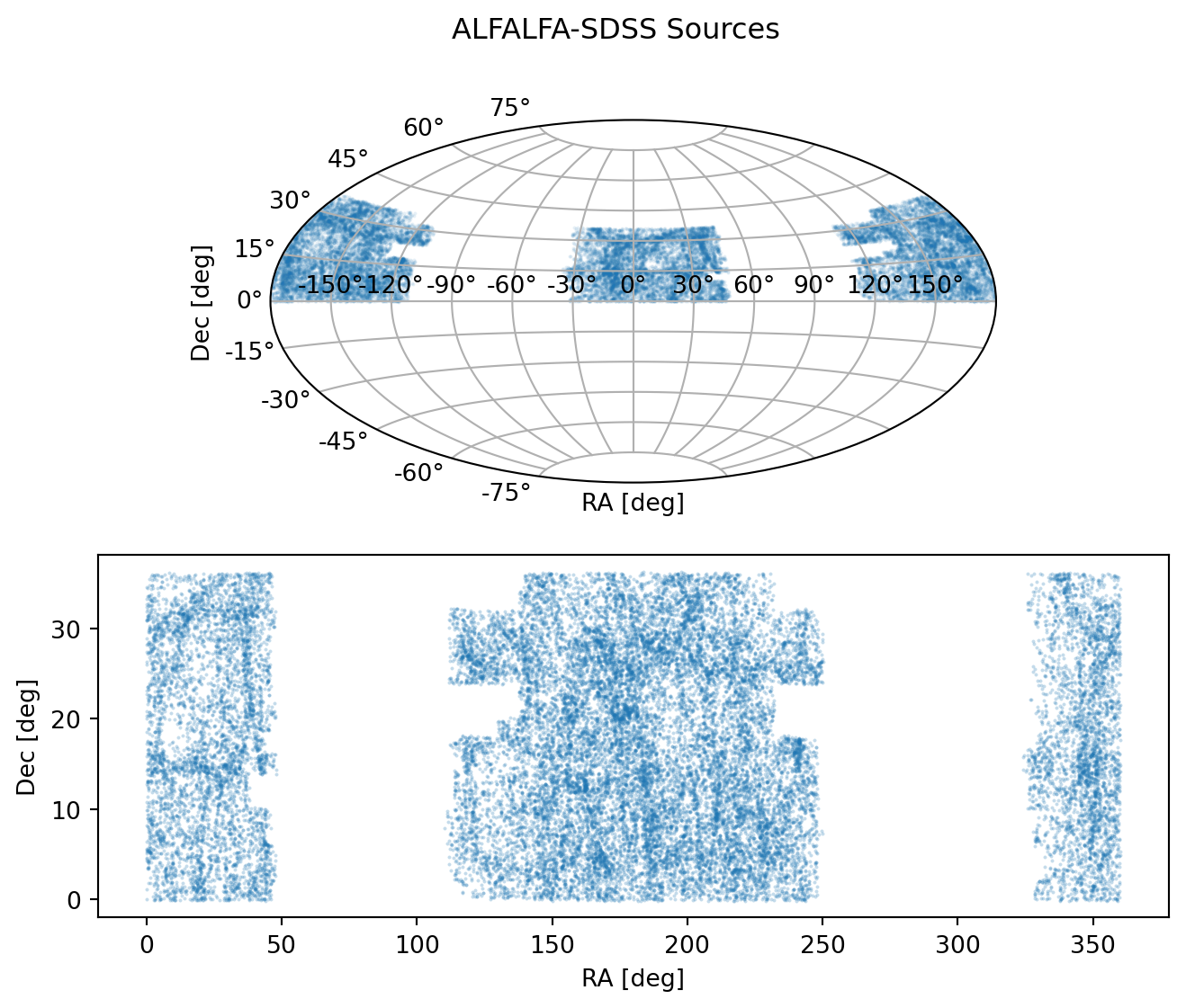
# zeropoint plot
data.sort("DEJ2000")
# convert spherical coordinates to cartesian
data["px"] = data["Dist"] * np.cos(data["WRAPPED_RA"]) * np.cos(data["WRAPPED_DE"])
data["py"] = data["Dist"] * np.sin(data["WRAPPED_RA"]) * np.cos(data["WRAPPED_DE"])
data["pz"] = data["Dist"] * np.sin(data["WRAPPED_DE"])
data["size"] = 1
num_plots = 4 # change number of plots here
dec_chunks = np.array_split(data["DEJ2000"], num_plots) # split the data into chunks
plt.figure(figsize=(num_plots*2, num_plots*2)) # matplotlib subplots
fig = make_subplots(rows=num_plots // 2, cols=num_plots // 2,
specs=[[{'type': 'scatter3d'}, {'type': 'scatter3d'}],
[{'type': 'scatter3d'}, {'type': 'scatter3d'}]])
row = 1
col = 1
for chunk, i in zip(dec_chunks, range(num_plots)):
# join chunk with rest of catalog to get all columns
chunk = Table(data = {"DEJ2000": chunk})
merged = join(chunk, data, keys="DEJ2000")
ascii.write(merged, f"dec{np.abs(np.min(merged["DEJ2000"])):.0f}to{np.max(merged["DEJ2000"]):.0f}.dat", format="commented_header", overwrite=True)
# matplotlib version
plt.subplot(num_plots // 2, num_plots // 2, i + 1, projection="polar")
plt.scatter(merged["WRAPPED_RA"], merged["Dist"], marker='.', s=1, alpha=0.5)
plt.xlabel(f"{np.min(merged["DEJ2000"]):.2f} < Dec < {np.max(merged["DEJ2000"]):.2f}")
# plotly version
px_merged = merged.to_pandas()
print(row, col)
fig.add_scatter3d(x=px_merged["px"], y=px_merged["py"], z=px_merged["pz"], row=row, col=col, mode="markers", marker=dict(size=px_merged["logMHI"], color=px_merged["imag"]))
if col >= num_plots // 2:
row += 1 # move to next row
col = 1 # restart the column
else:
col += 1
plt.suptitle(f"Redshift Plots: {num_plots} Splits")
plt.tight_layout()
fig.update_layout(margin=dict(l=20, r=20, t=20, b=20),
scene=dict(aspectmode="cube"))
# fig.show(renderer="browser")1 1
1 2
2 1
2 2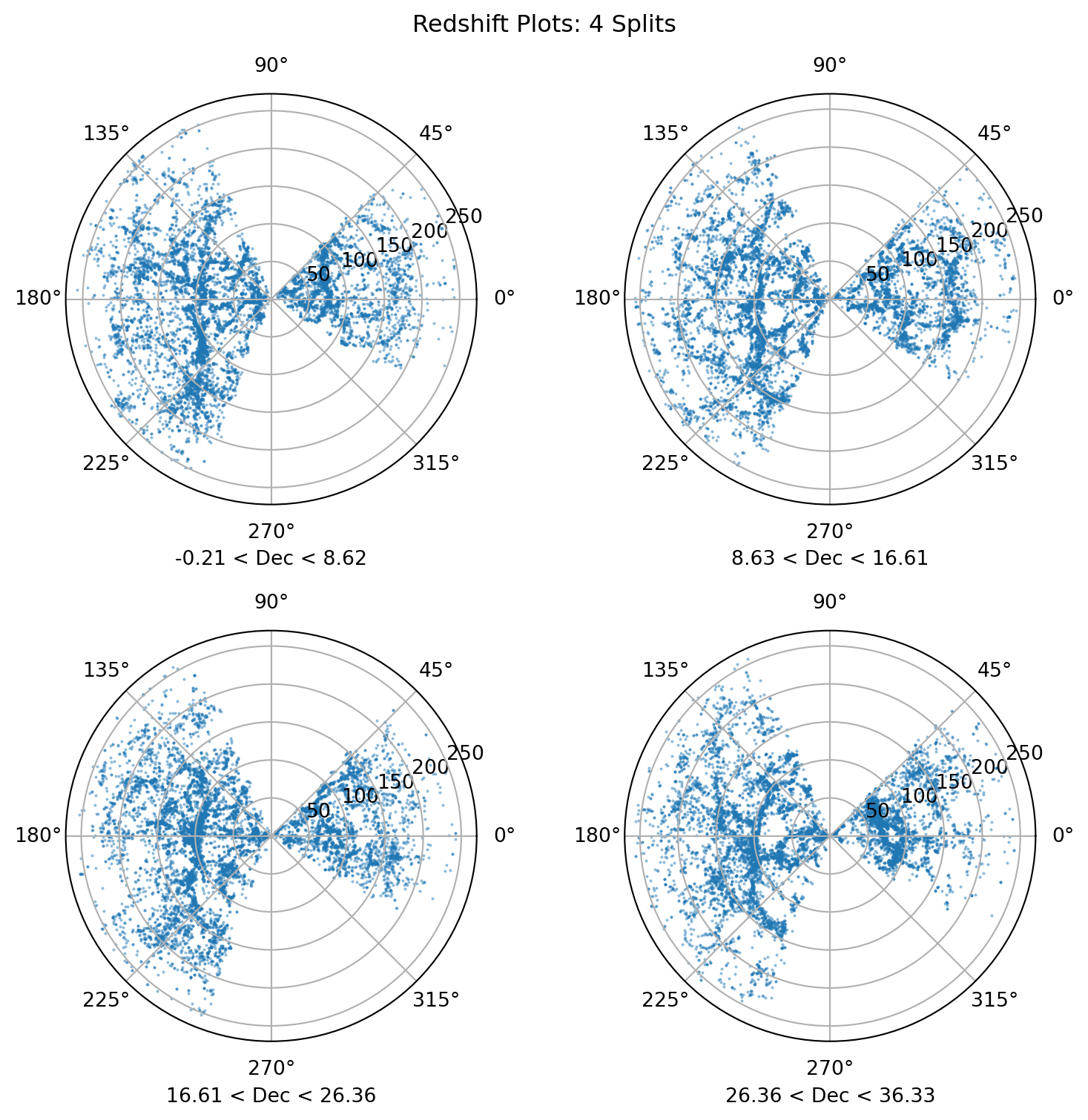
data.info()<Table length=31501>
name dtype unit format description class n_bad
---------- ------- ------------------- -------- -------------------------------------------------------------------------- ------------ -----
AGC int32 [1/749512] AGC catalog identifier MaskedColumn 0
Flag uint8 [0/3] Photometry flag (1) MaskedColumn 0
ObjID int64 Optical counterpart SDSS DR15 object identifier MaskedColumn 1863
RAJ2000 float64 deg {:10.6f} [0.003/360] Right Ascension (J2000) (2) MaskedColumn 0
DEJ2000 float64 deg {:9.5f} [-0.21/36.4] Declination (J2000) (2) MaskedColumn 0
RVel int16 km / s [-430/17823] HI profile midpoint heliocentric radial velocity MaskedColumn 0
Dist float32 Mpc {:5.1f} [0.3/260] Distance from Haynes+, 2018, J/ApJ/861/49 MaskedColumn 0
e_Dist float32 Mpc {:4.1f} [0/30.9] Uncertainty in Dist MaskedColumn 0
gext float32 mag {:5.2f} [0.02/4.44]? Foreground Galactic extinction in SDSS g band (3) MaskedColumn 1863
iext float32 mag {:5.2f} [0.01/2.28]? Foreground Galactic extinction in SDSS i band (3) MaskedColumn 1863
b/a float32 {:5.2f} [0.05/1]? Axial ratio b/a from SDSS r band MaskedColumn 1863
e_b/a float32 {:6.2f} [0.01/865]? Uncertainty in b/a (4) MaskedColumn 1863
imag float32 mag {:5.2f} [9.58/30.89]? SDSS i band cmodel magnitude MaskedColumn 1863
e_imag float64 mag {:8.2f} [0.01/42134.68]? Uncertainty in imag (4) MaskedColumn 1863
Dprop str5 Derived properties (table 2) MaskedColumn 0
Sloan str5 Display the online SDSS DR16 for the nearest object MaskedColumn 0
Ag float32 mag {:5.2f} [0/1.91]? g band internal extinction factor (1) MaskedColumn 3234
Ai float32 mag {:5.2f} [0/0.99]? i band internal extinction factor (1) MaskedColumn 3234
iMAG float32 mag {:6.2f} [-24/-10]? Corrected absolute i band magnitude (2) MaskedColumn 3234
e_iMAG float32 mag {:5.2f} [0.02/86]? Uncertainty in iMAG MaskedColumn 3234
g-i float32 mag {:5.2f} [-1.97/3.8]? Corrected (g-i) color (2) MaskedColumn 3234
e_g-i float32 mag {:6.2f} [0.03/220.3]? Uncertainty in g-i MaskedColumn 3234
logMsT float32 log(solMass) {:5.2f} [4.49/12.45]? log Taylor method stellar mass (3) MaskedColumn 3234
e_logMsT float32 log(solMass) {:6.2f} [0.02/158]? Uncertainty in logMsT MaskedColumn 3234
logMsM float32 log(solMass) {:5.2f} [4.4/11.94]? log McGaugh method stellar mass (3) MaskedColumn 2203
e_logMsM float32 log(solMass) {:5.2f} [0.01/1.66]? Uncertainty in logMsM MaskedColumn 2203
logMsG float32 log(solMass) {:5.2f} [7.37/11.69]? log GSWLC-2 derived stellar mass MaskedColumn 16776
e_logMsG float32 log(solMass) {:5.2f} [0/0.25]? Uncertainty in logMsG MaskedColumn 16776
logSFR22 float32 log(solMass.yr**-1) {:5.2f} [-5.57/2.17]? log Star Formatation Rate from 22{mu}m unWISE photometry (4) MaskedColumn 7606
e_logSFR22 float32 log(solMass.yr**-1) {:5.2f} [0.01/3.6]? Uncertainty in logSFR22 MaskedColumn 7606
logSFRN float32 log(solMass.yr**-1) {:5.2f} [-3.53/7.88]? log Star Formatation Rate from GALEX NUV photometry (4) MaskedColumn 15387
e_logSFRN float32 log(solMass.yr**-1) {:5.2f} [0.02/28.03]? Uncertainty in logSFRN MaskedColumn 15388
logSFRG float32 log(solMass.yr**-1) {:5.2f} [-2.94/1.47]? log Star Formatation Rate from GSWLC-2 MaskedColumn 16776
e_logSFRG float32 log(solMass.yr**-1) {:5.2f} [0.0/1.08]? Uncertainty in logSFRG MaskedColumn 16776
logMHI float32 log(solMass) {:5.2f} [3.76/10.94] Haynes+, 2018, J/ApJ/861/49 log HI mass MaskedColumn 0
e_logMHI float32 log(solMass) {:5.2f} [0.0/1.12] Uncertainty in logMHI MaskedColumn 0
WRAPPED_RA float64 deg {:10.6f} [0.003/360] Right Ascension (J2000) (2) MaskedColumn 0
WRAPPED_DE float64 deg {:9.5f} [-0.21/36.4] Declination (J2000) (2) MaskedColumn 0
px float64 Mpc {:5.1f} [0.3/260] Distance from Haynes+, 2018, J/ApJ/861/49 MaskedColumn 0
py float64 Mpc {:5.1f} [0.3/260] Distance from Haynes+, 2018, J/ApJ/861/49 MaskedColumn 0
pz float64 Mpc {:5.1f} [0.3/260] Distance from Haynes+, 2018, J/ApJ/861/49 MaskedColumn 0
size int32 Column 0# plotly interactive 3d map
fig = px.scatter_3d(data.to_pandas(), "px", "py", "pz", color="imag", size="logMHI", size_max=6, hover_name="AGC", hover_data=["RAJ2000", "DEJ2000", "Dist"])
fig.add_scatter3d(x=[0], y=[0], z=[0], name="Milky Way", marker=dict(size=0.015, color='blue'))
# fig.show(renderer="browser")def inset_position_plot(bg_data, ra_bounds, dec_bounds, x0, y0, width, height, loc1, loc2, ax):
minra, maxra = ra_bounds
mindec, maxdec = dec_bounds
mask = (bg_data["RAJ2000"] > minra) & (bg_data["RAJ2000"] < maxra) & (bg_data["DEJ2000"] > mindec) & (bg_data["DEJ2000"] < maxdec)
inset_data = data[mask]
# background plot
ax.scatter(bg_data["RAJ2000"], bg_data["DEJ2000"], marker=".", s=1, alpha=0.5)
ax.set_xlabel("RA [deg]")
ax.set_ylabel("Dec [deg]")
# create inset
ax_inset = ax.inset_axes([x0, y0, width, height])
ax_inset.scatter(inset_data["RAJ2000"], inset_data["DEJ2000"], c=inset_data["Dist"], s=1)
ax_inset.set_xticks([])
ax_inset.set_yticks([])
# ax_inset.set_colorbar()
mark_inset(ax, ax_inset, loc1=loc1, loc2=loc2, fc="none", ec="0.5")
# ax.set_title("Position Plot with Inset Colored by Distance")
returnfig, axs = plt.subplots(3, 3, figsize=(14,14))
inset_position_plot(data, (0, 50), (15, 90), 0.3, 0.3, 0.65, 0.65, 2, 3, axs[0][0])
inset_position_plot(data, (0, 50), (0, 20), 0.4, 0.4, 0.55, 0.55, 2, 3, axs[0][1])
inset_position_plot(data, (100, 150), (22, 33), 0.2, 0.01, 0.55, 0.55, 1, 2, axs[0][2])
inset_position_plot(data, (175, 250), (20, 90), 0.2, 0.01, 0.55, 0.4, 1, 2, axs[1][0])
inset_position_plot(data, (100, 175), (0, 14), 0.2, 0.45, 0.55, 0.50, 3, 4, axs[1][1])
inset_position_plot(data, (125, 200), (0, 14), 0.2, 0.45, 0.55, 0.50, 3, 4, axs[1][2])
inset_position_plot(data, (175, 250), (0, 14), 0.2, 0.45, 0.55, 0.50, 3, 4, axs[2][0])
inset_position_plot(data, (320, 360), (15, 90), 0.2, 0.01, 0.55, 0.4, 1, 2, axs[2][1])
inset_position_plot(data, (320, 360), (0, 20), 0.2, 0.01, 0.55, 0.4, 1, 2, axs[2][2])
# inset_position_plot(data, (320, 360), (0, 17), 0.2, 0.01, 0.55, 0.4, 1, 2) # bottom right
plt.suptitle("Possible Structures in ALFALFA-SDSS, Colored by Distance")
plt.tight_layout()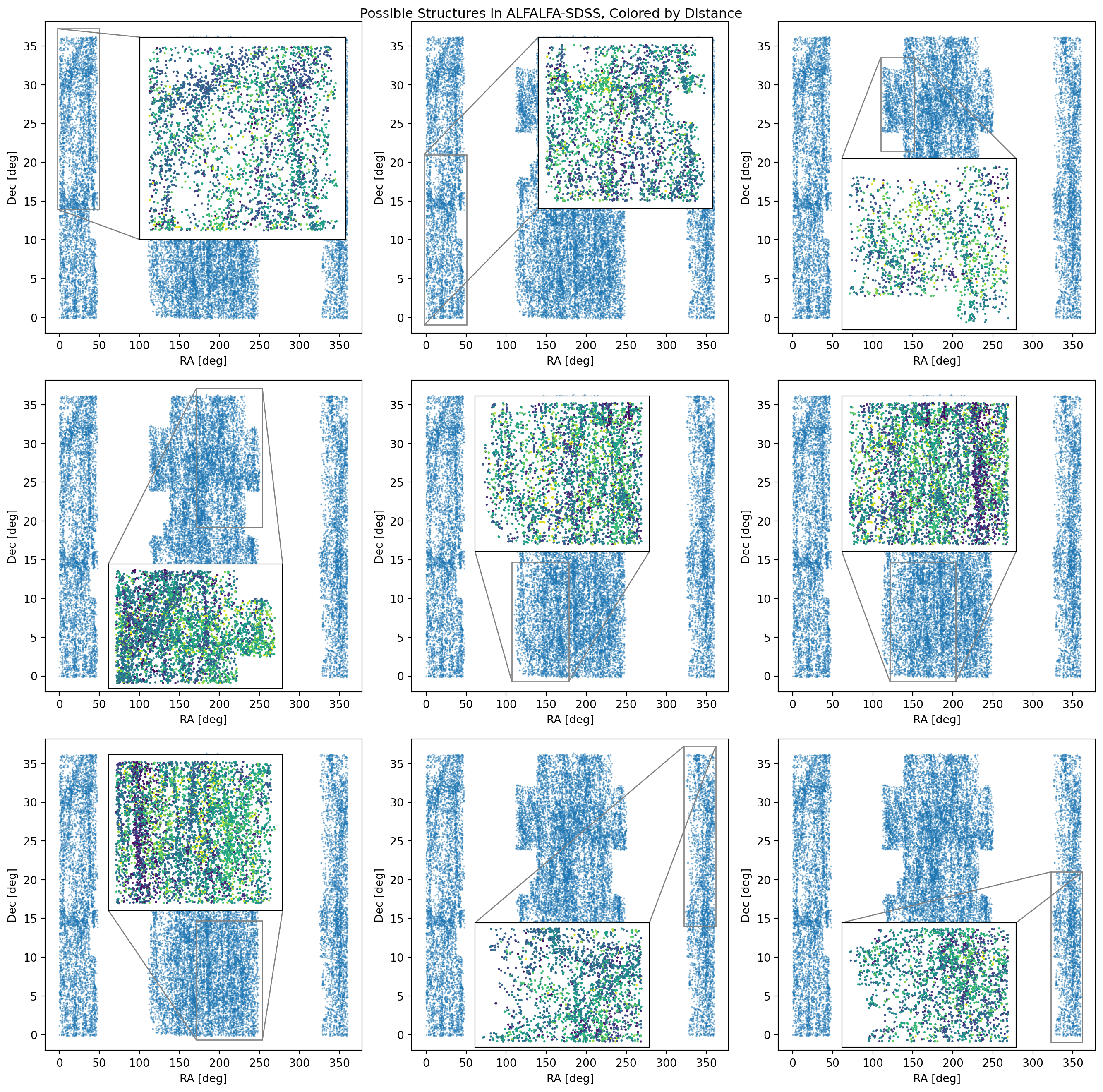
Interactive Structure Plot
# # plotly interactive 3d map
# fig = px.scatter(data.to_pandas(), "RAJ2000", "DEJ2000", size_max=1, opacity=0.25, hover_name="AGC", hover_data=["RAJ2000", "DEJ2000", "Dist"], color_continuous_scale=px.colors.sequential.Blues)
# fig.show()
# # plotly interactive 3d map
# fig = px.scatter(data.to_pandas(), "RAJ2000", "DEJ2000", color="Dist", size_max=1, opacity=0.25, hover_name="AGC", hover_data=["RAJ2000", "DEJ2000", "Dist"], color_continuous_scale=px.colors.sequential.Viridis)
# fig.show()
# Create a figure with subplots, linking the x and y axes
fig = make_subplots(
rows=1,
cols=2,
subplot_titles=('Plain', 'Colored by Distance'),
shared_xaxes=True,
shared_yaxes=True
)
# Add the first scatter plot to the first subplot
fig.add_trace(
go.Scatter(x=data["RAJ2000"], y=data["DEJ2000"], mode='markers', name='Data 1', marker=dict(
colorscale='Blues',
size=5,
opacity=0.25
)),
row=1,
col=1
)
# Add the second scatter plot to the second subplot
fig.add_trace(
go.Scatter(x=data["RAJ2000"], y=data["DEJ2000"], mode='markers', name='Data 2', marker=dict(
color=data["Dist"],
colorscale='Viridis',
size=5,
opacity=0.25
)),
row=1,
col=2
)
# Update layout for better appearance
fig.update_layout(
showlegend=False
)
fig.show()3D DisPerSE Output
# import pandas as pd
# import matplotlib.pyplot as plt
# import plotly.graph_objects as go
# df = pd.read_csv("simu_32_id.gad.NDnet_s3.52.up.NDskl.S010.a.segs", sep=" ", skiprows=[0,2]).rename(columns={"#U0": "U0"})
# u_list = df[["U0", "U1", "U2"]].to_numpy()
# v_list = df[["V0", "V1", "V2"]].to_numpy()
# fig = go.Figure()
# for start, end in zip(u_list, v_list):
# fig.add_trace(go.Scatter3d(
# x=[start[0], end[0]],
# y=[start[1], end[1]],
# z=[start[2], end[2]],
# mode='lines'
# ))
# fig.show()
# # fig.show(renderer="browser")2D DisPerSE Input
# import pandas as pd
# import matplotlib.pyplot as plt
# import numpy as np
# import astropy.units as u
# from astropy.coordinates import Angle
# # circle parameters
# center_x = 0
# center_y = 0
# radius = 10
# num_points = 200
# noise = np.random.uniform(0, 1, num_points)
# theta = np.linspace(0, 2 * np.pi, num_points)
# x = center_x + radius * np.cos(theta)
# y = center_y + radius * np.sin(theta)
# ra = x + noise
# dec = y + noise
# plt.scatter(ra, dec) # angle, distance
# df = pd.DataFrame({"ra": ra, "dec": dec}) # convert to degrees
# df.to_csv("circle_test.segs", sep=" ", index=False, header="# ra dec z")2D DisPerSE Output
# import pandas as pd
# import matplotlib.pyplot as plt
# import plotly.graph_objects as go
# import matplotlib.image as mpimg
# df = pd.read_csv("circle_test_nonperiodic.segs", sep=" ", skiprows=[0,2]).rename(columns={"#U0": "U0"})
# plt.figure(figsize=(12,6))
# plt.subplot(121)
# for i in range(len(df)):
# plt.plot([df["U0"].iloc[i], df["V0"].iloc[i]], [df["U1"].iloc[i], df["V1"].iloc[i]])
# plt.subplot(122)
# circle = pd.read_csv("test.survey_ascii", sep="\t")
# print(circle)
# plt.scatter(circle["ra"], circle["dec"])
# plt.tight_layout()
# plt.show()