Derive various important relationships that describe a blackbody radiation field.
Derive an expression for the number density of blackbody photons (photons per unit volume) with wavelength \(\lambda\) and \(d\lambda\). This differential should be expressed in terms \(d\lambda\).
Integrate the expression from a) over all wavelengths to obtain an expression for the total number density of blackbody photons. This results should include only numerical factors, fundamental constants, and the variable T (temperature).
Show that, for a blackbody, the average energy per photon is a simple relationship involving only a numerical factor, a single fundamental constant, and the variable T (temperature).
Answer: The blackbody spectral energy density \(u_\lambda\) for some \(\lambda+d\lambda\) is defined as \[u_\lambda d\lambda = \frac{4\pi}{c}B_\lambda d\lambda= \frac{8\pi hc}{\lambda^5}\left(\frac{1}{e^{hc/\lambda k T}-1}\right)d\lambda.\]
Addititonally, we know the a photon with wavelength \(\lambda\) has an energy described by \[E = hf = \frac{hc}{\lambda}\]
Dividing the blackbody spectral energy density by the photon energy will give us the number density of blackbody photons with wavelength \(\lambda\) and \(d\lambda\).
\[\boxed{n_\lambda d\lambda = \frac{u_\lambda d\lambda}{E} = \frac{8\pi}{\lambda^4}\left(\frac{1}{e^{hc/\lambda k T}-1}\right)d\lambda}\]
Integrating the right hand side over all wavelengths to find the total number density of blackbody photons results in the following integral.
\[\int_0^\infty\frac{8\pi hc}{\lambda^5}\left(\frac{1}{e^{hc/\lambda k T}-1}\right)d\lambda\]
Plugging this integral into Mathematica gives the following result
\[n = \int_0^\infty\frac{8\pi hc}{\lambda^5}\left(\frac{1}{e^{hc/\lambda k T}-1}\right)d\lambda = 16\pi\zeta(3)\left(\frac{kT}{ch}\right)^3\]
where \(\zeta(3)\) is the Riemann zeta function which has an approximate value of 1.20206. Thus our total number density of blackbody photons is
The total blackbody energy density over all wavelengths is \[u = aT^4, \quad a = \frac{4\sigma}{c} = 7.566\cdot10^{-16}\frac{\text{J}}{\text{m}^2 \text{K}^4}\]
If we divide the total blackbody energy density by our number density for blackbody photons found above, we should get the average energy per photon for a blackbody with temperature \(T\).
where the vertical optical depth is airmass dependent.
\[\tau_\lambda = \tau_{\lambda,0}\sec\theta\]
Once \(\tau_{\lambda,0}\) has been found, we can use either measured intensity and corresponding angle to determine the specific intensity before atmospheric attenuation.
In this problem you will use the values of density and opacity at various points near the surface of a model star to calculate the optical depth. The model is that of a 1 Solar mass star with \(T_{eff} = 5504\) K. The data in stellar-opacity.dat (on Moodle) shows physical values in the outer 3.3% of the star’s radius; the surface of the star is at \(r=7.1\times10^8\) m. We will use simple numerical integration to determine the optical depth in each region of the model. Recall that optical depth is defined by the relation Examining the data in the table, we see that we are given 42 model layers in the outer regions of the star. As one moves inward from the “surface” of the star to the interior, the values of \(\rho\) and \(\kappa\) change. We can determine the value of tau in each region by beginning with the outermost layer and working our way inward. To do this, we will apply the “Trapezoidal Rule”, a simple but effective numerical integration technique. The values of \(\tau\) in each subsequent layer can be found by applying the relation
where \(i\) and \(i+1\) designate adjacent zones in the model. Find the optical depth at each point by numerically integrating the relation for tau using the trapezoidal rule as provided.
Using the software package of your choice, create six plots:
kappa vs radius
rho vs radius
tau vs radius
Temperature vs radius
tau vs temperature
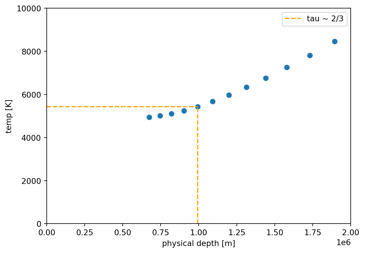
temperature vs physical depth into star
Estimate graphically the depth that one “sees” as the “surface” of this model star by zooming in on the appropriate region of plot #6. Include a zoom and your numerical estimate for the depth in (km).
Answer: The code below calculates the optical depth using the trapezoidal rule numerical integration for \(\tau_{i+1}\).
from astropy.io importasciiimport astropy.units as uimport matplotlib.pyplot as pltdata =ascii.read("stellar-opacity.dat")m =1* u.M_sunt_eff =5504* u.Kr =7.1E8* u.mtau_values = [0]tau =0for i inrange(len(data) -1): tau1 = tau - (data["kappa"][i] * data["rho"][i] + data["kappa"][i +1] * data["rho"][i +1]) /2* (data["r"][i +1] - data["r"][i]) tau = tau1 tau_values.append(tau)data["tau"] = tau_valuesdata["physical_depth"] = np.ones(len(data)) * r.value - data["r"]# eddington approximationdata["temp"] = (0.75* t_eff **4* (data["tau"] + (2/3))) ** (1/4)# plotting relationships# kappa vs radiusplt.figure(figsize=(8,10))plt.subplot(3,2,1)plt.scatter(y = data["kappa"], x = data["r"])plt.xlabel("radius [m]")plt.ylabel("kappa [m^2/kg]")# rho vs radiusplt.subplot(3,2,2)plt.scatter(y = data["rho"], x = data["r"])plt.xlabel("radius [m]")plt.ylabel("rho [kg/m^3]")# tau vs radiusplt.subplot(3,2,3)plt.scatter(y = data["tau"], x = data["r"])plt.xlabel("radius [m]")plt.ylabel("tau")# temp vs radiusplt.subplot(3,2,4)plt.scatter(y = data["temp"], x = data["r"])plt.xlabel("radius [m]")plt.ylabel("temp [K]")# tau vs tempplt.subplot(3,2,5)plt.scatter(y = data["tau"], x = data["temp"])plt.xlabel("temp [K]")plt.ylabel("tau")# temp vs physical depthplt.subplot(3,2,6)plt.scatter(y = data["temp"], x = data["physical_depth"])plt.xlabel("physical depth [m]")plt.ylabel("temp [K]")plt.subplots_adjust(wspace=0.5, hspace=0.5)plt.show()
The code below finds the value of \(\tau\) closest to 2/3, which corresponds to the optical depth we “see” as the “surface” and plots vertical and horizontal lines corresponding to the approximate physical depth and temperature, respectively.