import numpy as np
import astropy.units as u

# b)
Y = 16.854 - 5 * np.log10(49.59E3) + 5
X = -2.96
P = 1.1
M = X * P + Y
print(M)

# c)
m = 5 * np.log10(1.62E6) - 5 + M
print(m)
-4.878970541455551
21.168604531257603\[M_{F814W} = X \cdot (P/days) + Y\]
What does this recasting imply the absolute magnitude should be for a Cepheid with a period of 1.1 days?
Predict the apparent magnitude of the HST F814W filter of a Cepheid variable in the Local Volume galaxy Leo P with the same oscillation period. Use the distance to Leo P determined by McQuinn et al. (2015).
You may assume reddening-free situations for the Cepheids, and neglect the Wesenheit indices.
Answer: Given the magnitude
import numpy as np
import astropy.units as u
# b)
Y = 16.854 - 5 * np.log10(49.59E3) + 5
X = -2.96
P = 1.1
M = X * P + Y
print(M)
# c)
m = 5 * np.log10(1.62E6) - 5 + M
print(m)-4.878970541455551
21.168604531257603The Zwicky Transient Facility (ZTF) has revolutionized our understanding of pulsating stars. It has now discovered the majority of known pulsators of multiple classes. The manuscript by Chen et al. (2020) presents the ZTF catalog of pulsating stars. Read the manuscript to learn about the many types of pulsating stars.
If you’d rather start from presorted data, text files with the Table 2 data are provided for each pulsating star type are provided on Moodle.
Answer: If we measure the magnitude
from astropy.io import ascii
import matplotlib.pyplot as plt
data = ascii.read("https://content.cld.iop.org/journals/0067-0049/249/1/18/revision1/apjsab9caet2_mrt.txt")

cepI = data.group_by("Type").groups[1]
cepII = data.group_by("Type").groups[2]
RRab = data.group_by("Type").groups[7]
RRc = data.group_by("Type").groups[8]
D = data.group_by("Type").groups[3]
# plot r-band mag vs period for all stars
# color and label by star type
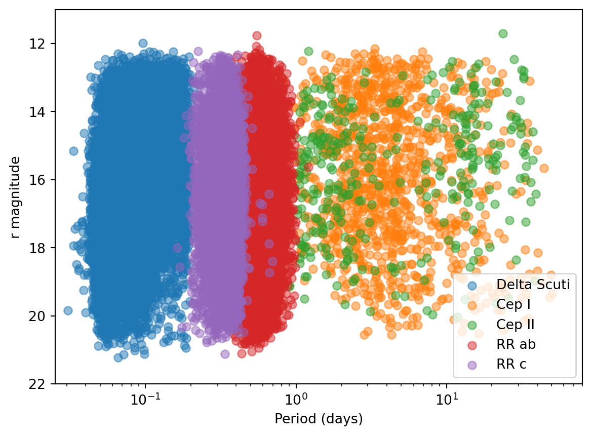
# log x axis, limits 0.025 to 80 days, linear magnitude axis, from 22 to 11
plt.scatter(D["Per"], D["rmag"], label = "Delta Scuti", alpha = 0.5)
plt.scatter(cepI["Per"], cepI["rmag"], label = "Cep I", alpha = 0.5)
plt.scatter(cepII["Per"], cepII["rmag"], label = "Cep II", alpha = 0.5)
plt.scatter(RRab["Per"], RRab["rmag"], label = "RR ab", alpha = 0.5)
plt.scatter(RRc["Per"], RRc["rmag"], label = "RR c", alpha = 0.5)
plt.xlabel("Period (days)")
plt.ylabel("r magnitude")
plt.legend()
plt.xscale("log")
plt.xlim(0.025, 80)
plt.ylim(22, 11)