The relationships for the Jeans mass, the Jeans length, and the free-fall timescale are fundamental. In this problem, you will explore these relationships over a range of physical properties. Consider a cloud of pure molecular hydrogen. Create two plots to demonstrate the behaviors of these fundamental relations:
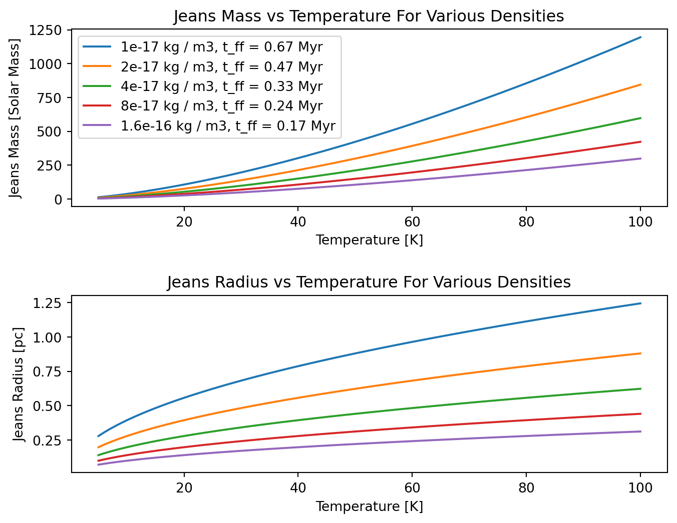
Jeans Mass versus temperature: Plot the Jeans Mass (in units of Solar masses) versus temperature over the range 5 K \(\leq T \leq\) 100 K. Show curves for five different densities, starting at \(1\times10^{-17}\) kg m\(^{-3}\) and increasing by a factor of two for each subsequent calculation. Clearly label each curve with its value of density and also with its characteristic free-fall timescale (in units of Myr).
Jeans Length versus temperature: Plot the Jeans Length (in units of pc) versus temperature over the range 5 K \(\leq T \leq\) 100 K. Show curves for five different densities, starting at \(1\times10^{-17}\) kg m\(^{-3}\) and increasing by a factor of two for each subsequent calculation. Clearly label each curve with its value of density and also with its characteristic free-fall timescale (in units of Myr).
In a few sentences describe the trends you observe in each of the plots you created.
Answer: The Jeans Mass increases as temperature increases, but increases more rapidly for lower density material. The lowest density material also has the longest time to collapse. The Jeans Radius increases more slowly at higher temperatures across all densities, however the Jeans Radius for lower density material is higher than the Jeans Radius for the higher density material across all temperatures.
How do these astronomers investigate the IMF? (Describe data, models, etc.)
What do they conclude about the IMF?
How do their results compare to what we talked about in class?
Answer: We read: Early Enrichment Population Theory at High Redshift by Blackwell and Bregman, published in The Astrophysical Journal on January 20, 2025.
The visible galaxies and stars in a galaxy cluster cannot have produced the measured ICM metallicity. In order to have the observed intracluster medium metallicity of glaxy clusters, a theory exists that says a population of stars must have existed at high redshifts that populated the clusters with the missing metals. Previous work argued the IMF of this theory must be flatter than lower redshift IMFs, but they didn’t have that high precision. This work used supernovae, delay time distributions, and luminosity functions of galaxy clusters to derive two best-fit IMFs that are flatter than standard IMFs.
Their model can successfully produce the observed ICM metallicity and agrees with observations. Interestingly, the model also predicts a rise in the Type Ia supernova rate at increasing redshift.
In class, we only talked about the interstellar medium. This paper introduced the idea of an intrcluster medium, which is like the ISM but on much larger scales. Overall, it seems the process for determining the two is just a scaled mapping; instead of looking at clusters of stars, like we do for the ISM, we look at clusters of galaxies.